Inverse Complementary Error Function Calculator
Online calculator for computing the inverse complementary error function erfci(x)
Inverse Complementary Error Function Calculator
The Inverse Complementary Error Function
The inverse complementary error function erfci(x) computes quantiles of tail probabilities and is essential for statistical inference and critical values.
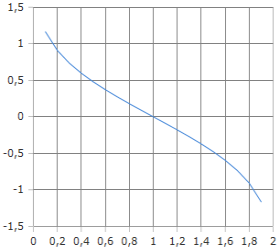
Inverse Complementary Error Function Curve
The curve shows the inverse of tail probabilities.
Mapping from probability to argument value.
What is the Inverse Complementary Error Function?
The inverse complementary error function erfci(x) is the inverse of the complementary error function:
- Definition: erfci(y) is the x such that erfc(x) = y
- Quantile Function: Computes critical values from tail probabilities
- Range: 0 ≤ y ≤ 2
- Application: Statistical hypothesis tests, critical values, confidence intervals
- Significance: Bridge between probability and normal quantiles
- Related to: Normal distribution quantiles, z-values
Critical Values and Statistical Applications
The inverse complementary error function is fundamental for statistical inference:
Critical Value Interpretation
- Tail Probability: erfci(α) is the critical value for tail probability α
- Normal Quantile: erfci(y) = √2 × Φ⁻¹(1 - y/2) for N(0,1)
- Significance Level: erfci(α) for α-level tests
- Confidence Limits: erfci(α/2) for (1-α)% confidence
Signal Detection
- Detection Thresholds: erfci applied to error probabilities
- Receiver Design: ROC curves and operating points
- False Alarm Rate: Converting probability to threshold
- Communication Systems: Bit error rate to SNR conversion
Applications of the Inverse Complementary Error Function
The inverse complementary error function is indispensable for modern statistics and engineering:
Hypothesis Testing
- Critical values for z-tests
- Significance thresholds (α-levels)
- Two-tailed and one-tailed tests
- Power analysis and sample sizing
Signal Processing
- Bit error rate (BER) analysis
- Detection threshold computation
- Noise immunity assessment
- Channel capacity calculations
Quality Assurance
- Acceptance sampling
- Process control limits
- Risk assessment (defect rates)
- Reliability design
Numerical Analysis
- Confidence interval computation
- Bootstrap resampling
- Monte Carlo simulation
- Iterative numerical methods
Formulas for the Inverse Complementary Error Function
Inverse Function Definition
x is the value such that the complementary error function yields y
Tail Probability Interpretation
For standard normal distribution
Normal Distribution Relationship
Connection to normal quantile function Φ⁻¹
Inverse Relationship
Fundamental identity for inverse functions
Complementary Property
Related to inverse error function
Symmetry Property
Symmetry around the midpoint y = 1
Example Calculations for the Inverse Complementary Error Function
Example 1: Critical Value for Hypothesis Test
Question
- Standard normal test: N(0,1)
- Significance level: α = 0.05 two-sided
- Find: Critical z-value
Calculation
Example 2: Bit Error Rate in Communication
Problem
- Target bit error rate: BER = 10⁻⁵
- AWGN channel, BPSK modulation
- Relationship: BER = (1/2)erfc(√SNR)
Solution
Example 3: Calculator Default Value
Question
Analytical Solution
Inverse Complementary Error Function Values
| y (Probability) | erfci(y) | Significance | Application |
|---|---|---|---|
| 0.1 | 1.1631 | 90% CI | Moderate confidence |
| 0.05 | 1.6449 | 95% CI | Standard confidence |
| 0.02 | 2.0537 | 98% CI | High confidence |
| 0.01 | 2.3263 | 99% CI | Very high confidence |
| 0.001 | 3.0902 | 99.9% CI | Extreme confidence |
Mathematical Foundations of the Inverse Complementary Error Function
The inverse complementary error function erfci(x) is the inverse of the complementary error function and plays a crucial role in probability calculations and statistical inference. It bridges the gap between probability values and the argument values of the normal distribution.
Historical Development
The error function and its inverse were developed alongside normal distribution theory:
- Pierre-Simon Laplace (1812): Integral of Gaussian function
- Carl Friedrich Gauss (1830): Systematic development of normal theory
- William Thurston (1870): Tables of error function
- Modern era: Numerical algorithms and computational methods
Mathematical Properties
The inverse complementary error function has important analytical properties:
Analytical Properties
- Monotonicity: Strictly decreasing function
- Domain: 0 ≤ y ≤ 2
- Range: -∞ < erfci(y) < +∞
- Limits: erfci(0) = ∞, erfci(2) = -∞
Computational Aspects
- Relationship to erf⁻¹: erfci(y) = -erf⁻¹(y-1)
- Normal approximation: erfci(y) ≈ √2 Φ⁻¹(1-y/2)
- Numerical stability: Special care for extreme values
- Computational methods: Newton-Raphson iteration
Connections to Other Functions
The inverse complementary error function is related to many statistical functions:
Statistical Functions
- Normal quantiles: erfci(α) gives z-values for α significance
- Q-function inverse: Q⁻¹(α) = erfci(2α)/√2
- Inverse normal CDF: Φ⁻¹(p) related to erfci
- t-distribution: Critical values via normal approximation
Engineering Functions
- Bit error rate: BER analysis and computation
- Signal detection: Threshold determination
- Receiver design: Operating point selection
- Communication systems: Performance prediction
Applications in Modern Sciences
Statistics & Quality
- Hypothesis test critical values
- Confidence interval boundaries
- Process control limits
- Risk assessment and AQL curves
Engineering & Physics
- Signal-to-noise ratio calculations
- Detection threshold determination
- Reliability engineering
- Thermal and diffusion processes
Summary
The inverse complementary error function is a fundamental tool for converting probability values into statistical critical values and engineering thresholds. Its close relationship to the normal distribution makes it indispensable for hypothesis testing, confidence intervals, quality control, and signal processing applications. Understanding its properties and efficient computation is essential for statistical analysis and engineering design.
|
|
|
|